Data Science and Hadoop: Part 5, Benford's Law Analysis
Context
This is the last part of a 5 part series on analyzing data with PySpark:
- Data Science and Hadoop : Impressions
- Data Overview and Preprocessing
- Basic Structural Analysis
- Outlier Analysis
- Benford’s Law Analysis
Benford’s Law
Benford’s Law is an interesting observation made by physicist Frank Benford in the 30’s about the distribution of the first digits of many naturally occurring datasets. In particular, the distribution of digits in each position follows an expected distribution.
I will leave the explanation of why Benford’s law exists to better sources, but this observation has become a staple of forensic accounting analysis. The reason for this interest is that financial data often fits the law and humans, when making up numbers, have a terrible time picking numbers that fit the law. In particular, we’ll often intuit that digits should be more uniformly distributed than they naturally occur.
Even so, violation of Benford’s law alone is insufficient to cry foul. It’s only an indicator to be used with other evidence to point toward fraud. It can be a misleading indicator because not all datasets abide by the law and it can be very sensitive to number of observations.
Ranking by Goodness of Fit
It’s of interest to us to figure out if this payment data fits the law and, if so, are there any payers who do not fit the law in a strange way. That leaves us with the technical challenge of determining how close two distributions are so that we can rank goodness of fit. There are a few approaches to this problem:
They are two approaches, one statistical and one information-theoretic, that will accomplish similar goals: tell how close two distributions are together.
I chose to rank based on KL divergence, but I compute the $\chi^2$ test as well. I’ll quote briefly about Kullback-Leibler divergence to give a sense of what the ranking means:
The Kullback–Leibler divergence of Q from P, denoted $D_{KL}(P || Q)$ , is a measure of the information lost when Q is used to approximate P. The KL divergence measures the expected number of extra bits required to code samples from P when using a code based on Q, rather than using a code based on P. Typically P represents the “true” distribution of data, observations, or a precisely calculated theoretical distribution. The measure Q typically represents a theory, model, description, or approximation of P.
In our case, P is the expected distribution based on Benford’s law and Q is the observed distribution. We’d like to see just how much more “complex” in some sense Q is versus P.
The Benford Digit Distribution
For the first digit, Benford’s law states that the probability of digit $d$ occurring is .
There is a generalization beyond the first digit which can be used as well. The probability of digit $d$ occurring in the second digit is .
#Compute benford's distribution for first and second digit respectively
benford_1=np.array([0] + [math.log10(1+1.0/i) for i in xrange(1,10)])
benford_2=np.array([ sum( [ math.log10(1 + 1.0/(j*10 + i)) \
                            for j in xrange(1, 10) \
                          ]\
                        )\
                     for i in xrange(0,10)\
                   ]\
                  )
Implementation of Benford’s Law Ranking
The way we’ll approach this problem is to determine the first and second digit distributions of payments by payer/reason and rank by goodness of fit for the first digit. Then we’ll look at the top fitting and bottom fitting payers for a few different reasons and see if we can see any patterns. One caveat is that we’ll be throwing out data under the following scenarios:
- The payer/specialty does not have at least 400 payments
- The amount is less than $10 (therefore not having a second digit)
Obviously the second one may skew things as it throws out some data within a partition but not the whole partition. In real analysis, I’d find a way to include the data points.
#Return a numpy array of zeros of specified $length except at
#position $index, which has value $value
def array_with_value(length, index, value):
    arr = np.zeros(length)
    arr[index] = value
    return arr

#Perform chi-square test between an expected probability
#distribution and a list of empirical frequencies.
#Returns the chi-square statistic and the p-value for the test.
def goodness_of_fit(emp_counts, expected_probabilities):
    #convert from probabilities to counts
    exp_distr = expected_probabilities*np.sum(emp_counts)
    return stats.chisquare(emp_counts, f_exp=exp_distr)


#For each (reason, payer) pair compute the first and second digit distribution
#for all payments.  Return a RDD with a ranked list based on likely goodness
#of fit to the distribution of first digits predicted by Benford's "Law".
def benfords_law(min_payments=350):
    """
    Benford's "law" is a rough observation that the distribution of numbers
    for each digit position of certain data fits a specific distribution.
    It holds for quite a bit real-world data and, thus, has become of
    interest to forensic accountants.

    This function computes the distribution of first and second digits for
    each (reason, payer) pair and ranks them by goodness of fit to
    Benford's Law based on the first digit distribution.
    In particular, the goodness of fit metric that it is ranked by is
    kullback-liebler divergence, but chi-squared goodness of fit test
    is also computed and the results are cached.
    """

    #We use this one quite a bit in reducers, so it's nice to have it handy here
    sum_values = lambda x,y:x+y

    #Project out the reason, payer, amount, and amount_str, throwing
    #away amounts < 10 since they don't have 2nd digits.  This probably
    #skews the results, so in real-life, I'd not throw out entries so
    #cavalierly, but for the purpose of simplicity, I've done it here.

    #Also, we're pulling out the first and second digits here
    reason_payer_amount_info = sqlContext.sql("""select reason
                                                      , payer
                                                      , amount
                                                      , amount_str
                                                 from payments
                                              """)\
                                    .filter(lambda t:len(t[0]) > 3
                                                 and t[2] > 9.99\
                                           ) \
                                    .map(lambda t: ( (t[1], t[0]) \
                                                   ,dict( payer=t[1]\
                                                        , reason=t[0] \
                                                        , first_digit=t[3][0] \
                                                        , second_digit=t[3][1] \
                                                        )\
                                                   )\
                                        )
    reason_payer_amount_info.take(1)

    #filter out the reason / payer combos that have fewer payments than
    #the minimum number of payments
    reason_payer_count = reason_payer_amount_info.map(lambda t: (t[0],1)) \
                                                 .reduceByKey(sum_values) \
                                                 .filter(lambda t: \
                                                    t[1] > min_payments
                                                        )

    #inner join with the reason/payer's that fit the count requirement
    #and annotate value with the num payments
    reason_payer_digits = \
      reason_payer_amount_info.join(reason_payer_count) \
                              .map(lambda t: (t[0] \
                                             , annotate_dict(join_lhs(t)\
                                                            , 'num_payments'\
                                                            , join_rhs(t)\
                                                            )\
                                              )\
                                   )
    #compute the first digit distribution.
    #First we count each of the 9 possible first digits, then we translate
    #that count into a vector of dimension 10 with count for digit i
    #in position i.  We then sum those vectors, thereby getting the
    #full frequency per digit.
    first_digit_distribution = \
      reason_payer_digits.map(lambda t: ( (t[0], t[1]['first_digit'] ) , 1) ) \
                         .reduceByKey(sum_values) \
                         .map(lambda t: (t[0][0]\
                                        , array_with_value(10\
                                                          , int(t[0][1])\
                                                          , t[1]\
                                                          )\
                                        )\
                              ) \
                         .reduceByKey(sum_values)
    #same thing with the 2nd digit
    second_digit_distribution = \
      reason_payer_digits.map(lambda t: ( (t[0], t[1]['second_digit']) , 1) ) \
                         .reduceByKey(sum_values) \
                         .map(lambda t: (t[0][0]\
                                        , array_with_value(10\
                                                          , int(t[0][1])\
                                                          , t[1]\
                                                          )\
                                        )\
                              ) \
                         .reduceByKey(lambda x,y:np.array(x) + np.array(y))

    #We join the two, compute the goodness of fit based on chi-square test
    #and the distance from benford's distribution based on kl divergence.
    #Finally we sort by kl-divergence ascending (good fits come first).
    return first_digit_distribution\
            .join(second_digit_distribution) \
            .map(lambda t : ( t[0]\
                            , dict( payer=t[0][0] \
                                  , reason=t[0][1] \
                                  , first_digit_distr=join_lhs(t) \
                                  , second_digit_distr=join_rhs(t) \
                                  , first_digit_fit = \
                                      goodness_of_fit(join_lhs(t)[1:10] \
                                                     , benford_1[1:10] \
                                                     ) \
                                  , second_digit_fit = \
                                      goodness_of_fit(join_rhs(t), benford_2) \
                                  , kl_divergence = \
                                      stats.entropy( benford_1[1:10]\
                                                   , join_lhs(t)[1:10]\
                                                   )\
                                  ) \
                             ) \
                 ) \
            .map(lambda t : (t[1]['kl_divergence'], t[1]) )\
            .sortByKey(True) \
            .map(lambda t : ( (t[1]['payer'], t[1]['reason']), t[1]) )

benford_data = benfords_law(400)
#Plot the distribution of first and second digit side-by-side for a set of payers.
def plot_figure(title,entries):
num_rows = len(entries)
fig, axes = plt.subplots(nrows=len(entries), ncols=2, figsize=(12,12))
fig.tight_layout()
plt.subplots_adjust(top=0.91, hspace=0.55, wspace=0.3)
fig.suptitle(title, size=14)
bar_width = .4
for i,entry in enumerate(entries):
first_ax = axes[i][0]
first_digit_distr = entry[1]['first_digit_distr'][1:10]
sample_label_1 = \
"""$\chi$={}, $p$={}, kl={}, n={}"""\
.format( locale.format('%0.2f'\
, float(entry[1]['first_digit_fit'][0])\
) \
, locale.format('%0.2f'\
, float(entry[1]['first_digit_fit'][1])\
)\
, locale.format('%0.2f'\
, float(entry[1]['kl_divergence'])\
)\
, int(np.sum(first_digit_distr))\
)
first_digit_distr = first_digit_distr/np.sum(first_digit_distr)
first_ax.bar(np.arange(1,10) ,first_digit_distr, alpha=0.35\
, color='blue', width=bar_width, label="Sample"\
)
first_ax.bar(np.arange(1,10)+bar_width ,benford_1[1:10]\
, alpha=0.35, color='red', width=bar_width\
, label='Benford')
first_ax.set_xticks(np.arange(1,10))
first_ax.legend()
first_ax.grid()
first_ax.set_ylabel('Probability')
first_ax.set_title("{} First Digit\n{}"\
.format(entry[0][0].encode('ascii', 'ignore')\
, sample_label_1\
)\
)
second_ax = axes[i][1]
second_digit_distr = entry[1]['second_digit_distr']
sample_label_2 = \
'$\chi$={}, $p$={}, n={}'\
.format(locale.format('%0.2f'\
, float(entry[1]['second_digit_fit'][0])\
) \
, locale.format('%0.2f'\
, float(entry[1]['second_digit_fit'][1])\
)\
, int(np.sum(second_digit_distr))\
)
second_digit_distr = second_digit_distr/np.sum(second_digit_distr)
second_ax.bar(np.arange(0,10) ,second_digit_distr, alpha=0.35\
, color='blue', width=bar_width, label="Sample")
second_ax.bar(np.arange(0,10) + bar_width,benford_2, alpha=0.35\
, color='red', width=bar_width, label='Benford')
second_ax.set_xticks(np.arange(0,10))
second_ax.legend()
second_ax.grid()
second_ax.set_ylabel('Probability')
second_ax.set_title("{} Second Digit\n{}"\
.format(entry[0][0].encode('ascii', 'ignore')\
, sample_label_2\
)\
)
#Take n-worst or best (depending on t) entries for reason based on goodness
# of fit for benford's law and plot the first/second digit distributions
#versus benford's distribution side-by-side as well as the distribution
#of kl-divergences.
def benford_summary(reason, data = benford_data, n=5, t='best'):
raw_data = data.filter(lambda t:t[0][1] == reason).collect()
s = []
if t == 'best':
s=raw_data[0:n]
plot_figure("Top 5 Best Fitting Benford Analysis for {}"\
.format(reason)\
, s\
)
else:
s=raw_data[-n:][::-1]
plot_figure("Top 5 Worst Fitting Benford Analysis for {}"\
.format(reason)\
, s\
)
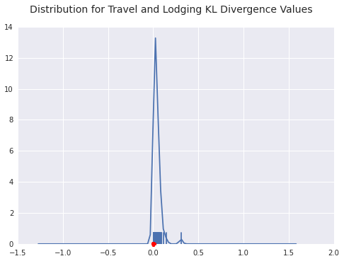
plot_outliers( [d[1]['kl_divergence'] for d in raw_data]\
, [d[1]['kl_divergence'] for d in s]\
, reason + " KL Divergence"\
)Best and Worst Fitting Payers for Gifts
Pretty much across the board the p-values for the $\chi^2$ test were super weak, but the first 4 are a pretty good fit. The last one is interesting, that spike at the 6 digit is the kind of thing that are of interest to forensic accountants. I repeat, however, that this is not an indicator which can be used safely alone to level a charge of fraud.
# Gift Benford Analysis (Best)
benford_summary('Gift', t='best')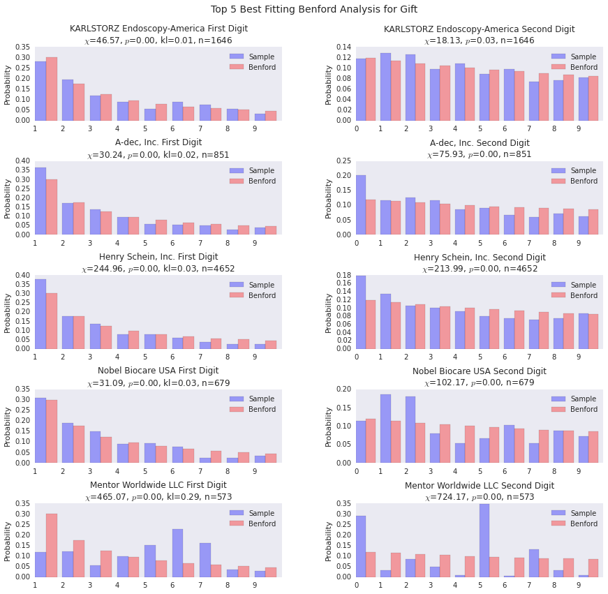
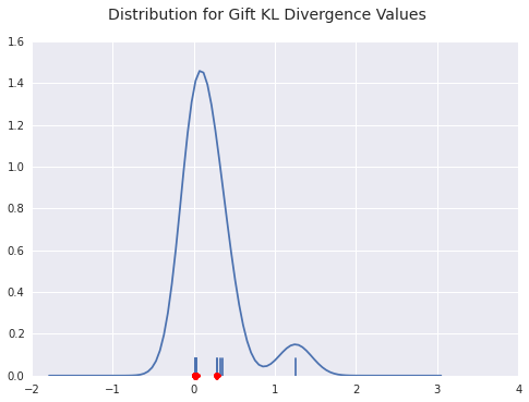
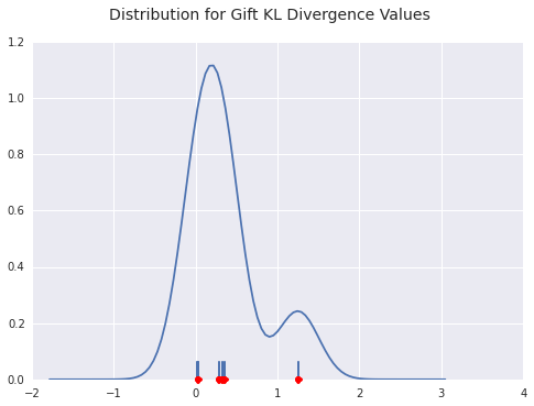
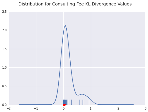
Below is the density plot for the Kullback-Leibler divergences for the top best fits. You can see there’s a clump at 0 and a clump a bit farther out, but no real outliers.
Now we look at the worst fitting gift payers. The lists overlap, as you can see, because there just aren’t that many organizations that pay more than 350 gifts out over the course of the year.
Two things that are interesting:
- Mentor Worldwide does not fit the decreasing probability distribution that we would expect. Many payers diverge from Benford’s law, but it’s interesting when they break the basic form of decreasing probabilities as digits progress from 1 through 9.
- Benco Dental Supply has a huge amount of payments starting with 1. This is likely an indication that they have a standard gift that they give out.
benford_summary('Gift', t='worst')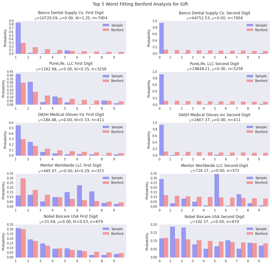
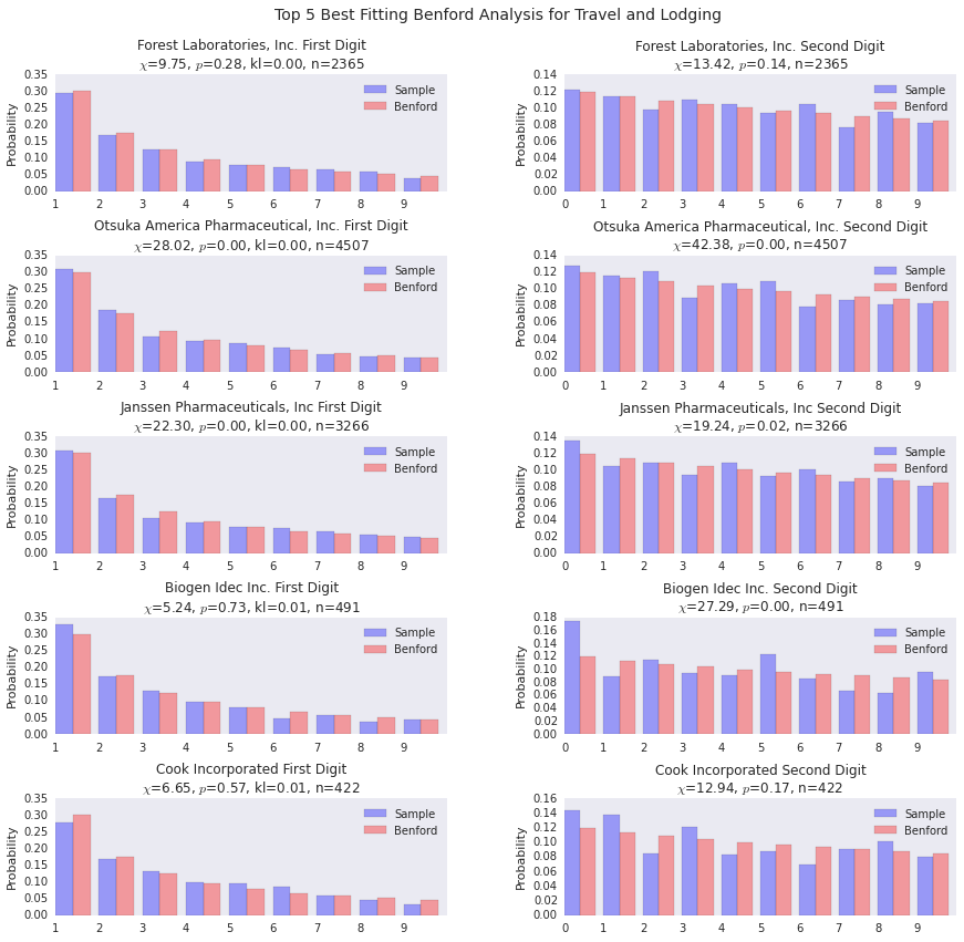
Best and Worst Fitting Payers for Travel and Lodging
# Travel and Lodging Benford Analysis
benford_summary("Travel and Lodging")
The top fitting payers for travel and lodging fit fairly well, so it’s certainly possible to fit the distribution well.
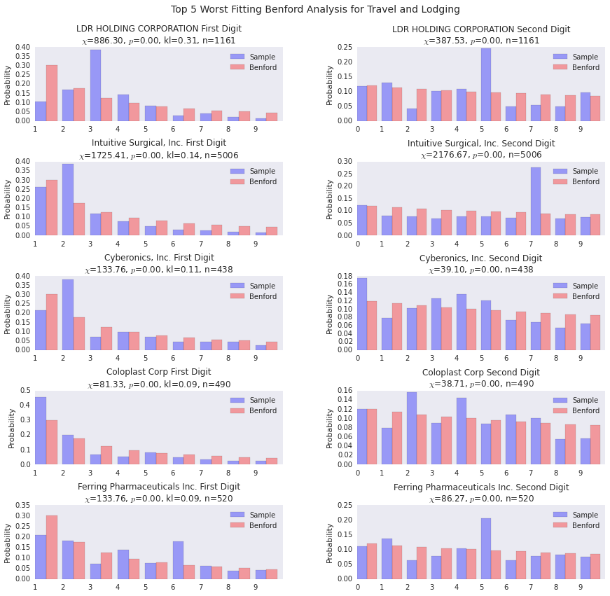
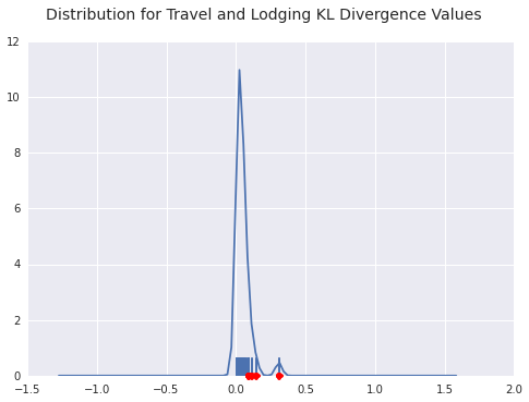
benford_summary("Travel and Lodging", t='worst')You can see a few payers diverging from the general form of Benford’s distribution here. LDR Holding is the outlier in terms of goodness of fit as you can see from the density plot below as well.
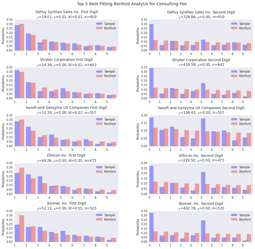
Best and Worst Fitting Payers for Consulting Fees
benford_summary("Consulting Fee")The good fits are pretty good.
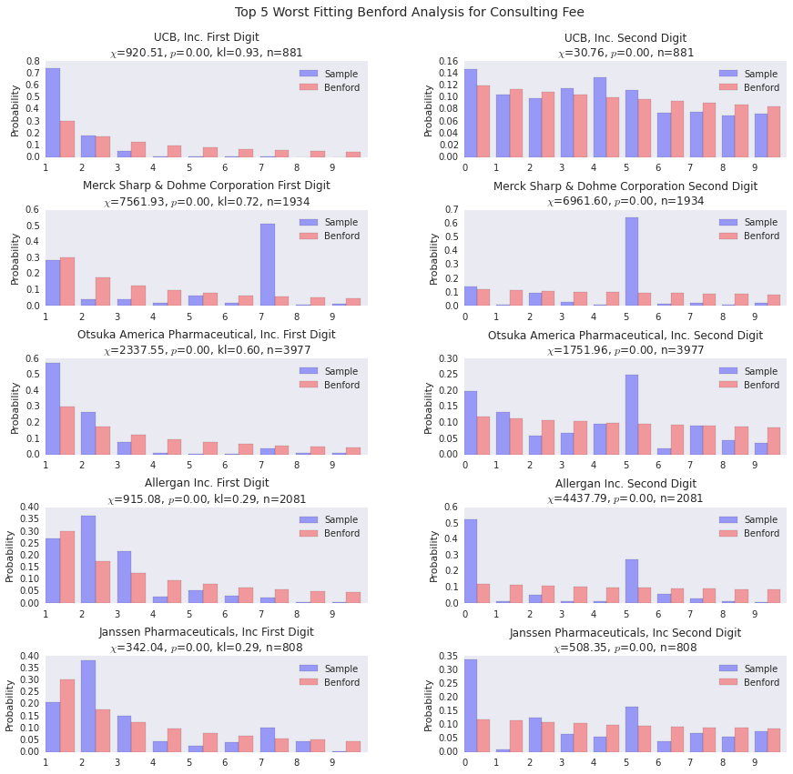
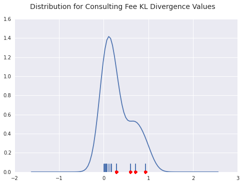
benford_summary("Consulting Fee", t='worst')For both UCB and Merck, we see a payer with a huge distribution of payments starting with 7. This indicates a standardized payment of some sort, I’d wager. The interesting thing about Merck is that the 1’s distribution is pretty spot on, the rest of the density gets pushed into 7.
Conclusion
This concludes the basic example of doing analytics with the Spark platform. General conclusions and impressions from this whole exercise can be found here.
Casey Stella 24 October 2014 Cleveland, OH