Data Science and Hadoop: Part 4, Outlier Analysis
Context
This is the fourth part of a 5 part series on analyzing data with PySpark:
- Data Science and Hadoop : Impressions
- Data Overview and Preprocessing
- Basic Structural Analysis
- Outlier Analysis
- Benford’s Law Analysis
Outlier Analysis
Generating summary statistics is very helpful for
- Understanding the overall shape of the data
- Looking at trends at the extreme (answering most, least, etc style questions)
One thing we’re doing when we’re looking for fishy things in data is looking to quickly zoom in on things which are outside of the norm. Furthermore, the aim is to automatically tag these as data is ingested so they can be acted on. This action can be raising an alert, logging a warning or generating a report, but ultimately we want a technique to find these outliers quickly and without human intervention.
Median Absolute Deviation
We’re looking to create a mechanism to rank data points by their likelihood of being an outlier along with a threshold to differentiate them from inliers.
The area of outlier analysis is a vibrant one and there are quite a few techniques to choose from. Ranging from the exotic, like fitting an elliptic envelope to the straightforward, like setting a threshold based on standard deviations away from the mean. For our purposes, we’ll choose a middle path, but be aware that there are book-length treatments of the subject of outlier analysis.
Median Absolute Deviation is a robust statistic used, as standard deviations, as a measure of variability in a univariate dataset. It’s definition is straightforward:
Given univariate data $X$ with $\tilde{x}=$median($X$), MAD($X$)=median({$\forall x_i \in X \lvert |x_i - \tilde{x}|$}).
As compared to standard deviation, it’s a bit more resilient to outliers because it doesn’t have a square weighing large values very heavily. Quoting from the Engineering Statistics Handbook:
The standard deviation is an example of an estimator that is the best we can do if the underlying distribution is normal. However, it lacks robustness of validity. That is, confidence intervals based on the standard deviation tend to lack precision if the underlying distribution is in fact not normal.
The median absolute deviation and the interquartile range are estimates of scale that have robustness of validity. However, they are not particularly strong for robustness of efficiency.
If histograms and probability plots indicate that your data are in fact reasonably approximated by a normal distribution, then it makes sense to use the standard deviation as the estimate of scale. However, if your data are not normal, and in particular if there are long tails, then using an alternative measure such as the median absolute deviation, average absolute deviation, or interquartile range makes sense.
In the implementation we’ll be taking guidance the Engineering Statistics Handbook and Iglewicz and Hoaglin. As such, define an outlier like so:
For a set of univariate data $X$ with $\tilde{x} =$ median($X$), an outlier is an element $x_i \in X$ such that $M_i = \frac{0.6745(x_i − \tilde{x} )}{MAD(X)} > 3.5$, where $M_i$ is denoted the modified Z-score.
Before we jump into the actual algorithm, we create some helper functions to make the code a bit more readable and allow us to display the outliers.
#Some useful functions for more advanced analytics

#Joins in spark take RDD[K,V] x RDD[K,U] => RDD[K, [U,V] ]
#This function returns U
def join_lhs(t):
    return t[1][0]

#Joins in spark take RDD[K,V] x RDD[K,U] => RDD[K, [U,V] ]
#This function returns V
def join_rhs(t):
    return t[1][1]

#Add a key/value to a dictionary and return the dictionary
def annotate_dict(d, k, v):
    d[k] = v
    return d

#Plots a density plot of a set of points representing inliers and outliers
#A rugplot is used to indicate the points and the outliers are marked in red.
def plot_outliers(inliers, outliers, reason):
    fig, ax = plt.subplots(nrows=1)
    sns.distplot(inliers + outliers, ax=ax, rug=True, hist=False)
    ax.plot(outliers, np.zeros_like(outliers), 'ro', clip_on=False)
    fig.suptitle('Distribution for {} Values'.format(reason), size=14)
Now, onto the implementation of the outlier analysis. But, before we start, I’d like to make a couple notes about the implementation and possible scalability challenges going forward.
We are partitioning the data by (payment reason, physician specialty). I do not want to analyze outliers based on a cohort of data across a whole reason, but rather I want to know if a point is an outlier for a given specialty and reason.
If a coarser partitioning strategy is taken or the amount of data per partition becomes very large, the median implementation may become a limiting factor scalability wise. There are a few things to do, including using a tighter implementation (numpy’s implementation could be tighter as of this writing) or a streaming estimate. Needless to say, this is something that bears some thought going forward.
#Outlier analysis using Median Absolute Deviation

#Using reservoir sampling, uniformly sample N points
#requires O(N) memory
def sample_points(points, N):
    sample = [];
    for i,point in enumerate(points):
        if i < N:
            sample.append(point)
        elif i >= N and random.random() < N/float(i+1):
            replace = random.randint(0,len(sample)-1)
            sample[replace] = point
    return sample

#Returns a function which will extract the median at location 'key'
#a list of dictionaries.
def median_func(key):
    #Right now it uses numpy's median, but probably a quickselect
    #implementation is called for as I expect this doesn't scale
    return lambda partition_value : ( partition_value[0]\
                                    , np.median(
                                        [ d[key] \
                                         for d in partition_value[1]\
                                        ]\
                                               )\
                                    )

#Compute the modified z-score for use by  as per Iglewicz and Hoaglin:
#Boris Iglewicz and David Hoaglin (1993),
#"Volume 16: How to Detect and Handle Outliers",
#The ASQC Basic References in Quality Control: Statistical Techniques
#, Edward F. Mykytka, Ph.D., Editor.
def get_z_score(reason_to_diff):
    med = join_rhs(reason_to_diff)
    if med > 0:
        return 0.6745 * join_lhs(reason_to_diff)['diff'] / med
    else:
        return 0

def is_outlier(thresh):
    return lambda reason_to_diff : get_mad(reason_to_diff) > thresh

#Return a RDD of a uniform random sample of a specified size per key
def get_inliers(reason_amount_pairs, size=2000):
    group_by_reason = reason_amount_pairs.groupByKey()
    return group_by_reason.map(lambda t : (t[0], sample_points(t[1], size)))


#Return the outliers based on Median Absolute Deviation
#See http://www.itl.nist.gov/div898/handbook/eda/section3/eda35h.htm
#for more info.
#The input key structure is reason_specialty => dict(amount
#                                                   , physician
#                                                   , payer
#                                                   , specialty
#                                                   )
def get_outliers(reason_amount_pairs, thresh=3.5):
    """
        This uses the median absolute deviation (MAD) statistic to find
        outliers for each reason x specialty partitions.

        Outliers are computed as follows:
        * Let X be all the payments for a given specialty, reason pair
        * Let x_i be a payment in X
        * Let MAD be the median absolute deviation, defined as
          MAD = median( for all x in X, | x - median(X)| )
        * Let M_i be the modified z-score for payment x_i, defined as
          0.6745*(x_i − median(X) )/MAD

        As per the recommendations by Iglewicz and Hoaglin, a payment is
        considered an outlier if the modified z-score, M_i > thresh, which
        is 3.5 by default.


        REFERENCE:
        Boris Iglewicz and David Hoaglin (1993),
        "Volume 16: How to Detect and Handle Outliers",
        The ASQC Basic References in Quality Control: Statistical Techniques,
        Edward F. Mykytka, Ph.D., Editor.
    """

    group_by_reason = reason_amount_pairs.groupByKey()

    #Filter by only reason/specialty's with more than 1k entries
    #and compute the median of the amounts across the partition.

    #NOTE: There may be some scalability challenges around median,
    #so some care should be taken to reimplement this if partitioning
    #by (reason, specialty) does not yield small enough numbers to
    #handle in an individual map function.
    reason_to_median = group_by_reason.filter(lambda t: len(t[1]) > 1000) \
                                      .map(median_func('amount'))

    #Join the base, non-grouped data, with the median per key,
    #consider just the payments more than the median
    #since we're looking for large money outliers and annotate
    #the dictionary for each entry x_i with the following:
    # * diff = |x_i - median(X)| in the parlance of the comment above.
    #   NOTE: Strictly speaking I can drop the absolute value since
    #         x_i > median(X), but I choose not to.
    # * median = median(X)
    #
    reason_abs_dist_from_median = \
        reason_amount_pairs.join(reason_to_median) \
                           .filter(lambda t : \
                              join_lhs(t)['amount'] > join_rhs(t)\
                                  ) \
                           .map(lambda t :\
                                 ( t[0]\
                                 , dict( diff=abs(\
                                      join_lhs(t)['amount'] - join_rhs(t)\
                                                 )\
                                       , row=annotate_dict(join_lhs(t) \
                                                          , 'median' \
                                                          , join_rhs(t) \
                                                          )\
                                       )\
                                 )\
                               )

    # Given diff cached per element, we need only compute the median
    # of the diffs to compute the MAD.
    #Remember, MAD = median( for all x in X, | x - median(X)| )
    reason_to_MAD = reason_abs_dist_from_median.groupByKey() \
                                               .map(median_func('diff'))
    reason_to_MAD.take(1)

    # Joining the grouped data to get both | x_i - median(X) |
    # and MAD in the same place, we can compute the modified z-score
    # , 0.6475*| x_i - median(X)| / MAD, and filter by the ones which
    # are more than threshold we can then do some pivoting of keys and
    #sort by that threshold to give us the ranked list of outliers.
    return reason_abs_dist_from_median\
              .join(reason_to_MAD) \
              .filter(is_outlier(thresh))\
              .map(lambda t: (get_z_score(t)\
                             , annotate_dict(join_lhs(t)['row']\
                                            , 'key'\
                                            , t[0]\
                                            )\
                             )\
                  ) \
              .sortByKey(False) \
              .map(lambda t: ( t[1]['key']\
                             , annotate_dict( t[1]\
                                            , 'mad'\
                                            , t[0]\
                                            )\
                             )\
                  )

#Filter the outliers by reason and return a RDD with just the outliers
#of a specified reason.
def get_by_reason(outliers, reason):
    return outliers.filter(lambda t: str.startswith(t[0].encode('ascii'\
                                                               , 'ignore'\
                                                               )\
                                                   ,reason\
                                                   )\
                          )

#Grab data using Spark-SQL and filter with spark core RDD operations
#to only yield the data we want, ones with physicians, payers and reasons
reason_amount_pairs = \
    sqlContext.sql("""select reason
                           , physician_specialty
                           , amount
                           , physician_id
                           , payer
                      from payments"""\
                  )\
              .filter(lambda row:len(row.reason) > 3 \
                              and len(row.physician_id) > 3\
                              and len(row.payer) > 3\
                     ) \
              .map(lambda row: ( "{}_{}".format( row.reason\
                                               , row.physician_specialty\
                                               )\
                             , dict(amount=row.amount\
                                   ,physician_id=row.physician_id\
                                   ,payer=row.payer\
                                   ,specialty=row.physician_specialty\
                                   )\
                             )\
                   )

#Get the outliers based on a modified z-score threshold of 3.5
outliers = get_outliers(reason_amount_pairs, 3.5)
#Get a sample per specialty/reason partition
inliers = get_inliers(reason_amount_pairs)
Now that we have found the outliers per specialty/reason partition, and a sample of inliers, let’s display them so that we can get a sense of how sensitive the outlier detection is.
#display the top k outliers in a table and a distribution plot
#of an inlier sample along with the outliers rug-plotted in red
def display_info(inliers_raw, outliers_raw_tmp, reason, k=None):
    outliers_raw = []
    if k is None:
        outliers_raw = sorted(outliers_raw_tmp\
                             , key=lambda d:d[1]['amount']\
                             , reverse=True\
                             )
    else:
        outliers_raw = sorted(outliers_raw_tmp\
                             , key=lambda d:d[1]['amount']\
                             , reverse=True\
                             )[0:k]
    inlier_pts = []
    for i in [d[1] for d in inliers_raw]:
        for j in i:
            inlier_pts.append(j['amount'])
    outlier_pts= [d[1]['amount'] for d in outliers_raw]
    plot_outliers(inlier_pts[0:1500], outlier_pts, reason)

    print_table(['Physician','Specialty', 'Payer', 'Amount']\
               , [d[1]['physician_id'] for d in outliers_raw]\
               , [ [ d[1]['specialty'] \
                   , d[1]['payer'].encode('ascii', 'ignore') \
                   , '$' + locale.format('%0.2f', d[1]['amount'], grouping=True)\
                   ] \
                 for d in outliers_raw]\
               )
Food and Beverage Purchase Outliers
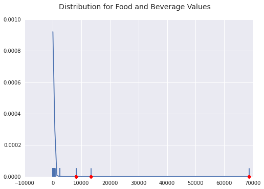
Let’s look at the top 4 outliers for Food and Beverage payments. I could have shown all of the outliers, but I found the first few to be the biggest bang for our buck in terms of interesting findings.
#outliers for food and beverage purchases
food_outliers = get_by_reason(outliers, 'Food and Beverage').collect()
food_inliers = get_by_reason(inliers, 'Food and Beverage').collect()
display_info(food_inliers, food_outliers, 'Food and Beverage', 4)
As we can see, the misclassified data from Teleflex is rearing its head again with a huge single payment for food. However, looking down the list, Biolase is paying quite a bit to some dentist for food.
| Physician | Specialty | Payer | Amount |
|---|---|---|---|
| 200720 | Allopathic & Osteopathic Physicians/ Surgery | Teleflex Medical Incorporated | $68,750.00 |
| 28946 | Dental Providers/ Dentist/ General Practice | BIOLASE, INC. | $13,297.15 |
| 28946 | Dental Providers/ Dentist/ General Practice | BIOLASE, INC. | $8,111.82 |
| 28946 | Dental Providers/ Dentist/ General Practice | BIOLASE, INC. | $8,111.82 |
Below is a density plot of outliers and a sample of inliers with a rug plot and the outliers marked in red. You can see how far along the tail of the densitiy plot the outliers here are. Most food and payment data hovers much closer to $0$.
Travel and Lodging Outliers
travel_outliers = get_by_reason(outliers, 'Travel and Lodging').collect()
travel_inliers = get_by_reason(inliers, 'Travel and Lodging').collect()
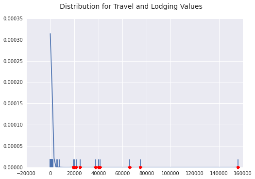
display_info(travel_inliers, travel_outliers, 'Travel and Lodging', 10)All I can say is that Physician 106320 travels far more than I do to get paid $155k in 2013. Hope that triple platinum on Delta is worth it. :)
| Physician | Specialty | Payer | Amount |
|---|---|---|---|
| 106320 | Allopathic & Osteopathic Physicians/ Psychiatry & Neurology/ Neurology | Boehringer Ingelheim Pharma GmbH & Co.KG | $155,772.00 |
| 472722 | Allopathic & Osteopathic Physicians/ Internal Medicine/ Nephrology | Merck Sharp & Dohme Corporation | $75,000.00 |
| 371379 | Allopathic & Osteopathic Physicians/ Orthopaedic Surgery | Exactech, Inc. | $65,798.00 |
| 198801 | Allopathic & Osteopathic Physicians/ Internal Medicine/ Cardiovascular Disease | Medtronic Vascular, Inc. | $41,232.80 |
| 382697 | Allopathic & Osteopathic Physicians/ Internal Medicine/ Nephrology | Genentech, Inc. | $39,978.80 |
| 169095 | Allopathic & Osteopathic Physicians/ Surgery | Medtronic Vascular, Inc. | $37,683.00 |
| 80052 | Allopathic & Osteopathic Physicians/ Family Medicine | Boehringer Ingelheim Pharma GmbH & Co.KG | $24,911.25 |
| 202461 | Allopathic & Osteopathic Physicians/ Thoracic Surgery (Cardiothoracic Vascular Surgery) | Covidien LP | $21,594.51 |
| 378722 | Allopathic & Osteopathic Physicians/ Internal Medicine | GlaxoSmithKline, LLC. | $20,112.40 |
| 243205 | Allopathic & Osteopathic Physicians/ Internal Medicine/ Interventional Cardiology | Medtronic Vascular, Inc. | $19,273.90 |
You can see on the density plot that the next nearest outlier is pretty far away and we have clumps of outliers around 20k and 40k. Interesting things to look into.
Consulting Fee Outliers
consulting_outliers = get_by_reason(outliers, 'Consulting Fee').collect()
consulting_inliers = get_by_reason(inliers, 'Consulting Fee').collect()
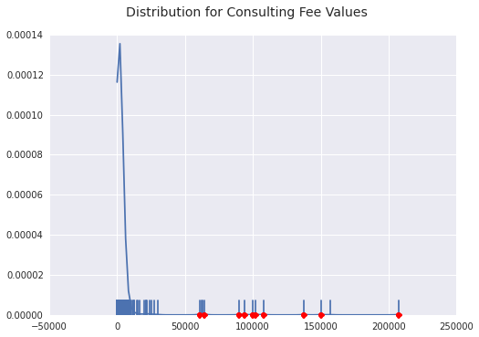
display_info(consulting_inliers, consulting_outliers, 'Consulting Fee', 10)Looking at consulting fee outliers, you can see some clumping, but most of the data is lower than 50k. That makes the 200k outlier from Teva all that much more interesting. Of course, none of this is any indication of wrong-doing, just interesting spikes in the data.
| Physician | Specialty | Payer | Amount |
|---|---|---|---|
| 104930 | Allopathic & Osteopathic Physicians/ Psychiatry & Neurology/ Neurology | Teva Pharmaceuticals USA, Inc. | $207,500.00 |
| 151515 | Other Service Providers/ Specialist | Alcon Research Ltd | $150,000.00 |
| 309376 | Allopathic & Osteopathic Physicians/ Internal Medicine | Teva Pharmaceuticals USA, Inc. | $137,559.67 |
| 231913 | Allopathic & Osteopathic Physicians/ Orthopaedic Surgery | Exactech, Inc. | $108,125.00 |
| 465481 | Allopathic & Osteopathic Physicians/ Internal Medicine/ Rheumatology | Vision Quest Industries Inc. | $102,196.09 |
| 409799 | Allopathic & Osteopathic Physicians/ Internal Medicine/ Endocrinology, Diabetes & Metabolism | Pfizer Inc. | $100,000.00 |
| 206227 | Allopathic & Osteopathic Physicians/ Orthopaedic Surgery | DePuy Synthes Sales Inc. | $93,750.00 |
| 436192 | Allopathic & Osteopathic Physicians/ Internal Medicine | Pfizer Inc. | $90,000.00 |
| 306965 | Allopathic & Osteopathic Physicians/ Psychiatry & Neurology/ Neurology | Teva Pharmaceuticals USA, Inc. | $64,125.00 |
| 163888 | Allopathic & Osteopathic Physicians/ Internal Medicine/ Cardiovascular Disease | Boehringer Ingelheim Pharmaceuticals, Inc. | $61,025.00 |
You can see most of the density is less than 20k, which makes that 200k outlier so interesting.
Gift Outliers
gift_outliers = get_by_reason(outliers, 'Gift').collect()
gift_inliers = get_by_reason(inliers, 'Gift').collect()
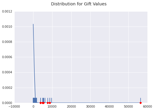
display_info(gift_inliers, gift_outliers, 'Gift', 10)Gifts, I think, are the most interesting payment reasons in this whole dataset. I am intrigued when a physician might get a gift versus an outright fee. I imagined, going in, that gifts would be low-value items, but the table clearly shows that dentists are getting substantial gifts. What is most interesting to me is that all of the top 10 outliers are dentists.
| Physician | Specialty | Payer | Amount |
|---|---|---|---|
| 225073 | Dental Providers/ Dentist/ General Practice | Dentalez Alabama, Inc. | $56,422.00 |
| 167931 | Dental Providers/ Dentist | DENTSPLY IH Inc. | $8,672.50 |
| 380517 | Dental Providers/ Dentist | DENTSPLY IH Inc. | $8,672.50 |
| 380073 | Dental Providers/ Dentist/ General Practice | Benco Dental Supply Co. | $7,570.00 |
| 403926 | Dental Providers/ Dentist | A-dec, Inc. | $5,430.00 |
| 429612 | Dental Providers/ Dentist | PureLife, LLC | $5,058.72 |
| 404935 | Dental Providers/ Dentist | A-dec, Inc. | $5,040.00 |
| 8601 | Dental Providers/ Dentist/ General Practice | DentalEZ, Inc. | $3,876.35 |
| 385314 | Dental Providers/ Dentist/ General Practice | Henry Schein, Inc. | $3,789.99 |
| 389592 | Dental Providers/ Dentist/ General Practice | Henry Schein, Inc. | $3,789.99 |
Up Next
Next, we look for anomalies in our payment data by using Benford’s Law. This is part of a broader series of posts about Data Science and Hadoop.
Casey Stella 24 October 2014 Cleveland, OH